GPU Water Flow & Hydrology Shaders in Delta Dynamics

In building Delta Dynamics, a low-poly ecosystem simulator, we wanted a world that felt hydrodynamically alive. Water shouldn’t just be a static visual plane; it should rain down, infiltrate the soil, accumulate in aquifers, flow down mountains, erode terrain, saturate soil, and form dynamic rivers and lakes that direct the growth of vegetation and the behaviors of AI entities.

Simulating this level of cellular hydrology in real time on a $100 \times 100$ grid is computationally heavy. If run on the CPU in JavaScript, updating 10,000 cells every frame alongside 3D rendering, entity AI, and local Web-LLM processing would quickly tank the frame rate.

To achieve a solid, lag-free 60 FPS in the browser, we offloaded the entire water cycle simulation to the GPU. By leveraging WebGL custom shaders via Three.js and a double-buffered Framebuffer Object (FBO) pipeline, we turned a heavy physics loop into a sub-millisecond graphics pass.

This post breaks down the mathematics of our discrete grid hydrology model, the double-buffering architecture, and the visual shader techniques used to render a beautiful, responsive low-poly water surface.

1. How Does GPU Hydrology Differ from Traditional Wave Shaders?

GPU-accelerated cellular hydrology simulates real, mass-conserving water volume and groundwater exchange on a discrete height grid rather than applying decorative surface vertex displacements (such as Gerstner waves). By evaluating shallow [SZ03] water diffusion and Darcy [Dar56]‘s subterranean permeability in WebGL fragment shaders, water realistically pools, infiltrates, and erodes terrain at 60 FPS.

The Coupled Surface and Subsurface Physics Model

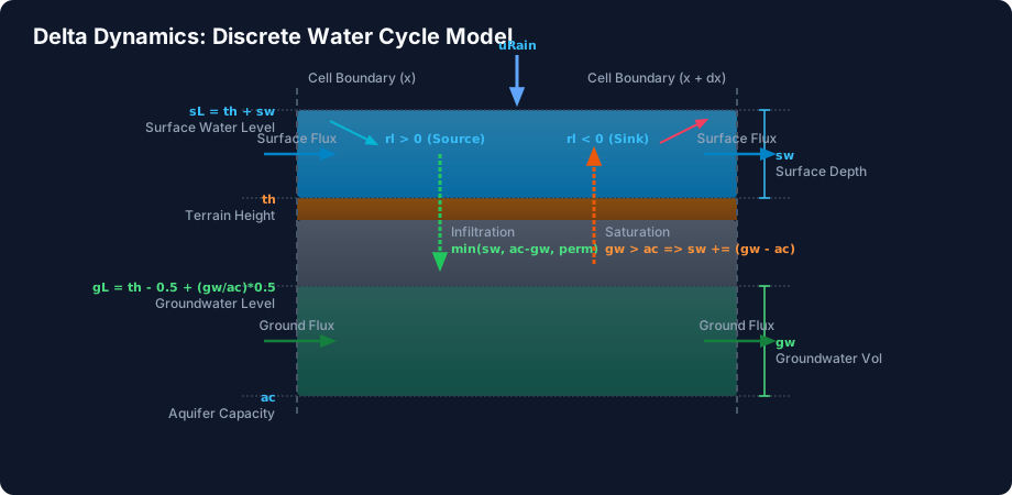
Most game water systems use simple wave-height maps that look nice but carry no physical volume. For an ecosystem simulator, we need mass-conserving volumetric water flow. We designed a coupled model comprising two main layers: Surface Water and Groundwater (Aquifers), connected by vertical fluxes.

Lateral Surface Water Flow (Diffusion & Flux Clamping)

We approximate the shallow water equations using a cell-centered, discrete height-based diffusion model. For each grid cell, we evaluate its 4-neighborhood (Up, Down, Left, Right).

The flow flux between a cell and its neighbor is driven by the difference in their total surface levels ($sL$), where $sL$ is the sum of the terrain elevation ($th$) and the surface water depth ($sw$):

$sL = th + sw$

The shader compares the local surface level with the neighbor’s level ($nSL$):

$sDiff = sL - nSL$

If $sDiff > 0$, water flows out to the neighbor; if $sDiff < 0$, water flows in. To prevent numerical instability and wild oscillations (where water sloshes back and forth indefinitely), we apply a safety flux clamp derived from the Courant [CFL28]-Friedrichs-Lewy (CFL) stability criterion in fluid dynamics ($\Delta t \le \frac{\Delta x}{c}$, where wave propagation speed $c = \sqrt{g \cdot h}$). On fixed grid cell resolutions ($\Delta x$) with discrete frame steps ($\Delta t$), unconstrained explicit Euler integration causes rapid divergence if outflux exceeds local cell volume. In our fragment shader simulation.frag.ts, outflow is capped at $30\%$ of the current cell’s water depth:

float sDiff = sL - nSL;
if (sDiff > 0.0001) {
    float f = sDiff * 0.22; // flow rate coefficient
    float clampedF = min(f, sw * 0.3); // clamp to prevent over-draining
    sDelta -= clampedF;
} else if (sDiff < -0.0001) {
    float f = -sDiff * 0.22;
    float clampedF = min(f, max(0.0, nWater.r - nSurface.r) * 0.3);
    sDelta += clampedF;
}

Physical Scope and Limitations of the 2D Heightfield Model

While discrete 2D heightfield shallow water simulation offers remarkable computational efficiency on web GPUs, engineers must recognize its inherent physical boundaries:

1. Single Height Surface Limitation: A heightfield $h(x, y)$ can only store one water surface elevation per grid coordinate. It cannot naturally represent true 3D fluid phenomena such as breaking waves, waterfalls with overhangs, caves, or complex turbulent vortex shedding.
2. Droplet Splashes and Phase Separation: Simulating fluid detachment (splashing droplets, mist, foam) requires 3D Eulerian grid solvers (e.g., Lattice Boltzmann or Navier-Stokes FLIP/PIC) or Lagrangian particle approaches (Smoothed Particle Hydrodynamics, SPH), which require significantly higher GPU memory bandwidth and compute shader capabilities.
3. Viscosity and Momentum Invariance: The diffusion model trades momentum advection (velocity fields) for computational stability, meaning inertial effects (like waves sloshing high up opposing canyon walls) are dampened compared to full Navier-Stokes formulations.

Subsurface Aquifer Flow (Darcy’s Law)

Beneath the surface, water permeates through porous soil layers (humus, sand, gravel, and rock). The groundwater level ($gL$) represents the hydraulic head inside the soil and is calculated based on the current groundwater volume ($gw$) relative to the aquifer’s capacity ($ac$):

$gL = th - 0.5 + \left(\frac{gw}{ac}\right) \times 0.5$

Groundwater flows laterally between adjacent cells following a simplified version of Darcy’s Law, where the flow rate is proportional to the hydraulic gradient ($gL - nGL$) and restricted by a much lower diffusion coefficient ($0.005$) compared to surface water ($0.22$):

float nGL = nSurface.r - 0.5 + (nAC > 0.0 ? (nWater.g / nAC) * 0.5 : 0.0);
float gDiff = gL - nGL;
if (gDiff > 0.0001) {
    float f = gDiff * 0.005;
    float clampedF = min(f, gw * 0.25);
    gDelta -= clampedF;
}

Vertical Fluxes: Infiltration & Saturation

Water moves vertically between the surface and the aquifer based on two physical processes:

1. Infiltration: Gravity forces surface water to sink into the soil. The rate of infiltration is dictated by the soil permeability ($perm$) of the top-most soil layer (e.g., pavement blocks infiltration, sand allows high infiltration):

   $amt = \min(sw, \min(ac - gw, 0.001 \times \frac{perm}{0.2}))$

2. Saturation & Exfiltration: If the aquifer is fully saturated ($gw > ac$), the soil cannot hold any more water. The excess groundwater is immediately pushed back to the surface ($sw += gw - ac; gw = ac$), creating puddles, springs, and waterlogged swamps.

2. WebGL Architecture: FBO Ping-Ponging

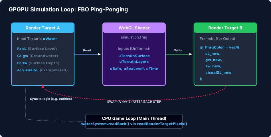
To run this cellular automata model on the GPU, we store the physical state of the grid in floating-point textures and run a double-buffered simulation loop.

Data Layout in Textures

We pack our grid variables into two main textures:

1. Water State Texture (uWater): A 2D Float texture storing the dynamic water quantities:
   • R: Surface Level ($sL$)
   • G: Groundwater volume ($gw$)
   • B: Surface Water depth ($sw$)
   • A: Visual extrapolated surface water level (used for rendering smooth shorelines)
2. Terrain Surface Texture (uTerrainSurface): A 2D Float texture storing static and dynamic terrain variables:
   • R: Pre-calculated total height ($th$)
   • G: River source/sink level ($rl$)
   • B: Top soil material index (used for permeability lookup)
   • A: Aquifer capacity ($ac$)

The Double-Buffering Loop

Since a shader cannot read from and write to the same texture simultaneously, we initialize two WebGL Render Targets (renderTargetA and renderTargetB).

In each simulation step, we:

1. Bind the current state (renderTargetA.texture) to the shader uniform uWater.
2. Render a full-screen quad using an orthographic camera into renderTargetB. The fragment shader computes the hydrology math and writes the new state to gl_FragColor.
3. Swap (ping-pong) the targets: renderTargetA becomes the new input, and renderTargetB becomes the next write destination.

This swap occurs inside waterSystem.ts:

public step(rain: number, inflow: number, seaLevel: number, time: number, ...) {
    this.computeMaterial.uniforms.uWater.value = this.renderTargetA.texture;
    this.computeMaterial.uniforms.uRain.value = rain;
    this.computeMaterial.uniforms.uInflow.value = inflow;
    this.computeMaterial.uniforms.uSeaLevel.value = seaLevel;
    this.computeMaterial.uniforms.uTime.value = time;

    const prevTarget = this.renderer.getRenderTarget();
    this.renderer.setRenderTarget(this.renderTargetB);
    this.renderer.render(this.scene, this.camera);
    this.renderer.setRenderTarget(prevTarget);

    // Swap Render Targets (Ping-Pong)
    const tmp = this.renderTargetA;
    this.renderTargetA = this.renderTargetB;
    this.renderTargetB = tmp;
}

Asynchronous CPU Readbacks

While the graphics card handles the physics math, CPU game logic still needs to know where the water is (e.g., so trees can consume groundwater, or so humans don’t drown). We implement readBack() which calls renderer.readRenderTargetPixels to transfer the float texture data back to CPU-accessible Float32Arrays. To keep performance high, this readback is throttled or run asynchronously to prevent blocking the GPU command pipeline.

3. Creating the Low-Poly Water Aesthetic

Simulated water is represented on a flat 2D grid texture. However, we want it to look like a stylized, volumetric low-poly surface. We achieve this with custom vertex and fragment shaders.

Vertex Shader: Smooth Wet-Neighbor Extrapolation

If we displacement-map a 3D grid mesh using raw water depths, dry cells would drop off sharply, resulting in jagged, blocky stair-step water edges. To make the water flow look organic:

1. Visual Extrapolation: In the simulation shader, we calculate a weighted average of wet neighbor heights and store this in the alpha channel (visualSL) of uWater.
2. Neighbor Level Averaging: In the vertex shader surface.vert.ts, we look up the 4 corner points of the quad and interpolate their visualSL values.
3. Dry-Vertex Sinking: If a vertex has no wet neighbors, we set its height to h - 0.05 (sinking it slightly below the terrain) to hide it.
4. Wave Animation: If the local water depth is greater than $0.05$, we add a small time-based sine wave to give the water a gentle ripple:

   GLSL

   Copy

   if (sw_interp > 0.05) {
     transformed.y += sin(uTime * 2.0 + (position.x + position.z) * 5.0) * 0.005;
   }

Fragment Shader: Depth Gradient, Shorelines, & Grid Lines

The fragment shader surface.frag.ts styles the water surface using depth-based gradients and custom highlights:

1. Depth-Based Color: We calculate the depth ($vDepth$) as the difference between the water surface height and the terrain height. We mix a vibrant sky blue (shallow) and a dark navy blue (deep) using smoothstep:

   GLSL

   Copy

   vec3 shallowColor = vec3(0.2, 0.5, 0.8);
   vec3 deepColor = vec3(0.02, 0.1, 0.3);
   vec3 waterColor = mix(shallowColor, deepColor, smoothstep(0.0, 0.5, vDepth));

2. Wet Edge Shorelines: Instead of a hard, ugly intersection line between the water mesh and the terrain, we fade the water color into the terrain color as $vDepth$ approaches zero. This gives the shoreline a smooth “wet sand” look.
3. Dynamic Source/Sink Pulses: When a river source (rl > 0) or drain (rl < 0) is active, we add a color pulse using sin(uTime * 3.0). Sources pulse a bright, cyan energy wave, while sinks pulse a red/orange whirlpool effect.
4. Procedural Grid Lines: To match the voxel/grid theme, we overlay subtle grid lines by taking the fractional coordinates: fract(vGridUv * 100.0).

4. Architectural Comparison: CPU Cellular Loop vs. GPU FBO Pipeline

The following matrix compares our double-buffered GPU shader approach against a traditional CPU JavaScript implementation across performance, memory footprint, and visual fidelity:

Frequently Asked Questions (FAQ)

Below are concise answers to key implementation questions regarding WebGL FBO ping-pong simulation and CPU-GPU synchronization:

What is FBO ping-pong buffering in Three.js?

FBO (Framebuffer Object) ping-pong buffering utilizes two alternating render targets (renderTargetA and renderTargetB). Because a WebGL shader cannot read from and write to the same texture simultaneously, Target A supplies the previous state as input while the fragment shader computes the new physical state onto Target B. The targets are swapped each frame, allowing continuous state evolution without data hazards.

How does the simulation prevent water from oscillating endlessly?

Numerical instability in discrete shallow water models is governed by the Courant-Friedrichs-Lewy (CFL) condition. In our shader, we enforce a strict flux clamp where outflow is capped at a maximum of 30% of the cell’s current water depth per frame, preventing artificial sloshing and infinite feedback loops.

How do CPU game entities interact with GPU-computed water?

Game entities require height queries to navigate terrain or consume groundwater. We implement an asynchronous readBack() pipeline that extracts raw pixel buffers via renderer.readRenderTargetPixels into typed arrays. Throttling readbacks to several frames per second ensures that GPU synchronization never stalls rendering.

5. Conclusion & Next Steps

By combining discrete cellular automata logic with GPGPU techniques, Delta Dynamics achieves a rich, physically active hydrological cycle in a standard web browser. Offloading the lateral diffusion and vertical infiltration equations to WebGL shaders guarantees that the water simulation stays incredibly fast, leaving the CPU free to focus on entity logic, pathfinding, and local LLM AI agents.

This hybrid approach demonstrates that modern browsers are fully capable of hosting complex, real-time physical simulations, bringing premium desktop-grade simulation mechanics directly to web applications.

Explore related high-performance graphics and simulation materials across our platform:

• Content Visualizations & Graph Engines
• University Course: Computer Simulation Course Materials
• WebGL Network Visualization & Graph Engines Architecture